 The Sacred Way
Route modeling of the Sacred Way between Miletos and Didyma
An open-source explanation using R code and libraries
Toby C. Wilkinson, Anja Slawisch
Introduction
This annex paper provides a walkthrough of the analytical procedures used to produce maps to understand the possible variations in route of the so-called Sacred Way between the ancient city of Miletos and its sometime-dependent oracle sanctuary at Didyma. It should be read in conjunction with and as support for the archaeologically and epigraphically oriented arguments in:
- Slawisch and Wilkinson (in prep). Processions, Propaganda and Pixels: Reconstructing the Sacred Way between Miletos and Didyma..
This analysis attempts to compare the generally-assumed or orthodox reconstruction of the Sacred Way between Miletos and Didyma with mathematically-derived or probability-based models of travel across a landscape. These models are called, variously, cost-surface, resistance or friction-surface analyses. They should, of course, be treated as heuristic rather than truly-predictive models, providing a visualization of “what we would expect”” if travel friction or cost were an important part of the decision-making in routing a particular path. Such cost factors can contribute to path generation either from rational decision-making (in the case of modern or ancient road building) or organically through a process akin to Darwinian selection (i.e. those taking the least-cost path are most successful from an energy/time-expenditure point of view).
Nature of this document
The static version you are currently reading was created on 2017-07-14, though the content has not changed since the date of the document described above.
NB: Procedures to create the necessary stages of analysis are shown here as R functions with the prefix
sw_, for clarity where similar procedures are preformed and to increase ease of re-use within this text and
by others.
# testing time of procedure
ptm <- proc.time()
This script relies on a number of libraries from the CRAN directory which must be installed before the full script can be run. Libraries are loaded before data import and calculations. It is recommended that R packages are installed manually before the script is run, as the set-up process can be different on different systems.
# Install the libraries It is recommended to
# install these packages manually per machine
# where possible, since some machines (e.g.
# Mac OS X) require a different version of
# RGDAL to function. See
# http://www.kyngchaos.com/software/frameworks
# for Mac OS X rgdal package.
# install.packages(c('knitr', 'sp', 'rgdal',
# 'plyr', 'dplyr', 'RColorBrewer',
# 'gdistance', 'maptools', 'rgeos'),
# repos='https://mirrors.ebi.ac.uk/CRAN/')
# Load the libraries
library("sp")
library("rgdal")
library("plyr")
library("dplyr")
library("RColorBrewer")
library("gdistance")
library("maptools")
library("rgeos")
# library(raster) #already required by other
# packages
Define fixed variables
The RMarkdown document assumes that it resides in a directory called panormos/analysis/sacredway and that relevant external files are to be found under the panormos/xxxxx.
# Script expects to find itself in
# panormos/analysis/sacredway or similar depth
# relative to other panormos data so that it
# can find panormos/gis-static etc.  Change
# this if the data directory structure is
# different.
working_dir <- "../../../"
Established default projection
Output for the maps will use the UTM 35N projection.
projection <- c(paste("+proj=utm +zone=35n ",
    "+datum=WGS84 +units=m ", "+no_defs +ellps=WGS84 ",
    "+towgs84=0,0,0", sep = ""))
Licencing of code/text
Since the aim of this paper is to facilitate replication of our results and provide the opportunity for future alternative interpretations, the information presented here is licensed using a Creative Commons (CC) BY licence which means that others are allowed to create derivative works provided the original source (i.e. this document) and the authors are cited.
GIS data/external files
This paper is designed to be used in association with geographical data which forms part of the Project Panormos archive. Those wishing to reproduce the analysis will need both the necessary R environment and the referenced data. Distributable data will be made available via http://www.projectpanormos.com/sacredway/ .
Load base spatial data
Load archaeological points-of-interest along the sacred way
point_sacred_gate <- readOGR(dsn = paste(working_dir,
    "gis-active/archaeology_base_features/sacred_way_reconstructions/",
    "points_along_the_sacred_way/miletos_sacredgate.gml",
    sep = ""), layer = "miletos_sacredgate", encoding = "UTF-8")

# Note that alter is a typo and needs to be
# corrected
point_didyma_altar <- readOGR(dsn = paste(working_dir,
    "gis-active/archaeology_base_features/sacred_way_reconstructions/",
    "points_along_the_sacred_way/didyma_alter_point.gml",
    sep = ""), layer = "didyma_alter_point", encoding = "UTF-8")

point_road_leaving_akron <- readOGR(dsn = paste(working_dir,
    "gis-active/archaeology_base_features/sacred_way_reconstructions/",
    "points_along_the_sacred_way/road_as_leaves_hills_point.gml",
    sep = ""), layer = "road_as_leaves_hills_point",
    encoding = "UTF-8")

point_cult_complex <- readOGR(dsn = paste(working_dir,
    "gis-active/archaeology_base_features/sacred_way_reconstructions/",
    "points_along_the_sacred_way/sw_point_archaic_cult_complex.gml",
    sep = ""), layer = "sw_point_archaic_cult_complex",
    encoding = "UTF-8")

point_nymph_complex <- readOGR(dsn = paste(working_dir,
    "gis-active/archaeology_base_features/sacred_way_reconstructions/",
    "points_along_the_sacred_way/sw_point_nymphs.gml",
    sep = ""), layer = "sw_point_nymphs", encoding = "UTF-8")

# also need a point for panormos!
# panormos_port_point.gml

point_panormos <- readOGR(dsn = paste(working_dir,
    "gis-active/archaeology_base_features/sacred_way_reconstructions/",
    "points_along_the_sacred_way/panormos_port_point.gml",
    sep = ""), layer = "panormos_port_point",
    encoding = "UTF-8")

points_lohmann <- readOGR(dsn = paste(working_dir,
    "gis-active/archaeology_base_features/lohmann_survey/",
    "sites_Lohmann.gml", sep = ""), layer = "sites_Lohmann",
    encoding = "UTF-8")
Load relatively fixed ancient structures
outline_ancient_structures <- readOGR(dsn = paste(working_dir,
    "gis-active/archaeology_base_features/sacred_way_reconstructions/",
    "points_along_the_sacred_way/ancient_structures.gml",
    sep = ""), layer = "ancient_structures", encoding = "UTF-8")
Load previous reconstructions and other useful contextual data
sacredway_schneider_south <- readOGR(dsn = paste(working_dir,
    "gis-active/archaeology_base_features/sacred_way_reconstructions/",
    "schneider/sw_line_alt_Schneider.gml", sep = ""),
    layer = "sw_line_alt_Schneider", encoding = "UTF-8")
sacredway_schneider_north <- readOGR(dsn = paste(working_dir,
    "gis-active/archaeology_base_features/sacred_way_reconstructions/",
    "schneider/sw_line_Schneider_MiletosSide.gml",
    sep = ""), layer = "sw_line_Schneider_MiletosSide",
    encoding = "UTF-8")
sacredway_wilski <- readOGR(dsn = paste(working_dir,
    "gis-active/archaeology_base_features/sacred_way_reconstructions/",
    "wilski1907/sw_line_wilksi_antikestrasse.gml",
    sep = ""), layer = "sw_line_wilksi_antikestrasse",
    encoding = "UTF-8")

## need to check projection
modern_major_roads <- readOGR(dsn = paste(working_dir,
    "gis-active/modern_features/modern_roads/",
    "major_roads.gml", sep = ""), layer = "major_roads",
    encoding = "UTF-8")

wilski_paths <- readOGR(dsn = paste(working_dir,
    "gis-active/modern_features/premodern_paths/",
    "wilski_paths.gml", sep = ""), layer = "wilski_paths",
    encoding = "UTF-8")
Load topographic models (DEMs)
# Needs to be changed to a standed DEM source,
# e.g. ASTER tile that anyone can download
# dem_modern <-
# raster(paste(working_dir,'gis-active-raster/topography/',
# 'aster_based_dem/dem_asterN37E27_modern_20m.tif',
# sep = ''))
# Load from standard ASTER source. Since the
# raw ASTER is distributed in LatLong
# projection, it needs to be
# reprojected/resampled to UTM to match the
# other parts of analysis, and cropped to a
# more managable area.
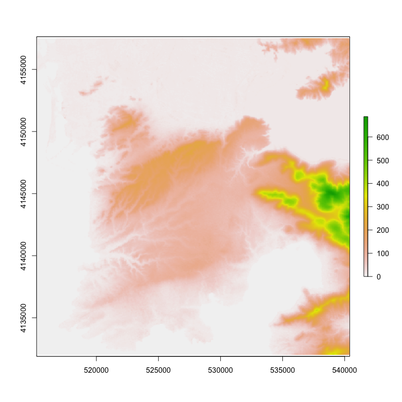
dem_modern <- raster(paste(working_dir, "gis-static/dem/",
"aster/ASTGTM2_N37E027/ASTGTM2_N37E027_dem.tif",
sep = ""))
sr <- "+proj=utm +zone=35 +datum=WGS84 +units=m +no_defs"
dem_modern <- projectRaster(dem_modern, crs = sr)
## Crop just to area of wider Ionia crop area
## set using UTM co-ordinates cropbox
## <-c(501150,569930,4102950,4180970)
cropbox <- c(515200, 540400, 4132000, 4157500) #4155000
dem_modern <- crop(dem_modern, cropbox)
plot(dem_modern)
# dem_ancient is now created programmatically
# from the modern dem
# A hi-res dem derived by digitizing the
# contours in Paul Wilski's 1903 map of the
# peninsula
dem_wilski <- raster(paste(working_dir, "gis-active-raster/topography/",
"wilski_dem/dem_wilskiso_landonly.tif", sep = ""))
# plot(dem_wilski)
# A polygon layer with the modern land shape
modern_land_shape <- readOGR(dsn = paste(working_dir,
    "gis-active/topography-vector/landshape/land_AD2000.gml",
    sep = ""), layer = "land_AD2000", encoding = "UTF-8",
    disambiguateFIDs = TRUE)

# Sea model according to Müllenhoff
sea_inundation_800BC <- readOGR(dsn = paste(working_dir,
    "gis-active/topography-vector/landshape/sea_inundation_800BC.gml",
    sep = ""), layer = "sea_inundation_800BC",
    encoding = "UTF-8")

panormos_harbour_800BC <- readOGR(dsn = paste(working_dir,
    "gis-active/topography-vector/landshape/",
    "panormos_harbour_800BC.gml", sep = ""), layer = "panormos_harbour_800BC",
    encoding = "UTF-8")

meander_delta_800BC <- readOGR(dsn = paste(working_dir,
    "gis-active/topography-vector/landshape/",
    "meander_delta_800BC.gml", sep = ""), layer = "meander_delta_800BC",
    encoding = "UTF-8")

meander_delta_300BC <- readOGR(dsn = paste(working_dir,
    "gis-active/topography-vector/landshape/",
    "meander_delta_300BC.gml", sep = ""), layer = "meander_delta_300BC",
    encoding = "UTF-8")

meander_delta_1BC <- readOGR(dsn = paste(working_dir,
    "gis-active/topography-vector/landshape/",
    "meander_delta_1BC.gml", sep = ""), layer = "meander_delta_1BC",
    encoding = "UTF-8")

modern_baffa_golu <- readOGR(dsn = paste(working_dir,
    "gis-active/topography-vector/landshape/",
    "baffagolu.gml", sep = ""), layer = "baffagolu",
    encoding = "UTF-8")
Load multispectral imagery from worldview
multi_spectral_image <- paste(working_dir, "gis-static/imagery/",
    "worldview2/052720256010_01/052720256010_01_P001_MUL/",
    "11SEP04091901-M2AS-052720256010_01_P001.TIF",
    sep = "")

if (file.exists(multi_spectral_image)) {
    worldview_multi <- brick(multi_spectral_image)
    worldview_multi[worldview_multi == 0] <- NA
} else {
    worldview_multi <- NULL
}
Transform land-shape and DEM data
Create land-shape vectors
The ancient land-shapes are calculated by ‘cutting out’ those areas of the modern land-shape which were sea in the past.
# Fix potential invalid geometries with
# 0-width buffer (i.e. self-intersections)
modern_land_shape <- gBuffer(modern_land_shape,
    byid = TRUE, width = 0)
sea_inundation_800BC <- gBuffer(sea_inundation_800BC,
    byid = TRUE, width = 0)
panormos_harbour_800BC <- gBuffer(panormos_harbour_800BC,
    byid = TRUE, width = 0)

ancient_land_shape_800BC <- gDifference(modern_land_shape,
    sea_inundation_800BC, byid = TRUE)
# take account of the additional area around
# Panormos which may have been sea rather than
# land
ancient_land_shape_800BC_panormos <- gDifference(ancient_land_shape_800BC,
    panormos_harbour_800BC, byid = TRUE)
Extract values for modern and ancient land-shapes from DEM rasters
Only the values from areas which were deemed to be land at certain dates should be included in the travel-distance calculations. To do this, the vector footprints of the land-shape at certain times are used to extract only these values.
# define function to clip a raster by a
# polygon shapefile
cliprasterbypolygon <- function(r, f, i = FALSE) {
    # only works if r (raster) and f (vector) are
    # in the same projection based on code answer
    # from Jeffrey Evans:
    # http://gis.stackexchange.com/questions/92221/
    # cr <- crop(r, extent(f), snap='in')
    cr <- r
    fr <- rasterize(f, cr)
    # plot(fr) plot(f, add=TRUE)
    lr <- mask(x = cr, mask = fr, inverse = i)
    return(lr)
}

dem_ancient <- cliprasterbypolygon(dem_modern,
    ancient_land_shape_800BC)
dem_modern <- cliprasterbypolygon(dem_modern,
    modern_land_shape)
# additional step required to ensure the Baffa
# Golu is indeed modelled as water (i.e. NA)
dem_modern <- cliprasterbypolygon(dem_modern,
    modern_baffa_golu, i = TRUE)


#### full wilski dem is very large (high res), so
#### only use the full version when ready to wait
#### dem_wilski_modern <- dem_wilski
#### dem_wilski_ancient <-
#### cliprasterbypolygon(dem_wilski,ancient_land_shape_800BC)
#### dem_wilski_prealluv <-
#### cliprasterbypolygon(dem_wilski,ancient_land_shape_800BC_panormos)

#### for now use stand-ins
dem_wilski_modern <- dem_modern
dem_wilski_ancient <- dem_ancient
dem_wilski_prealluv <- cliprasterbypolygon(dem_ancient,
    ancient_land_shape_800BC_panormos)
Crop DEM to area of interest for this analysis only
Only a discrete part of the DEM models is needed and to save processing time analysis and plots to the Milesian peninsula. The cropped area is hard-coded as cropbox below in UTM coordinates.
A second crop restricts the higher-resolution Wilksi-based DEM to a smaller area between Akkron and Didyma
## Whole peninsula crop area set using UTM
## co-ordinates
cropbox <- c(515200, 540400, 4132000, 4155000)

dem_modern <- crop(dem_modern, cropbox)
dem_ancient <- crop(dem_ancient, cropbox)

## Panormos close-up crop area set using UTM
## co-ordinates
panormos_cropbox <- c(518050, 527880, 4136500,
    4145500)
dem_wilski_modern <- crop(dem_wilski_modern, panormos_cropbox)
dem_wilski_ancient <- crop(dem_wilski_ancient,
    panormos_cropbox)
dem_wilski_prealluv <- crop(dem_wilski_prealluv,
    panormos_cropbox)
Export geographical data into re-usable GeoTIFF format (optionally)
# Export dem to packages
# writeRaster(dem_modern,
# filename='export/dem_modern.tif',
# overwrite=TRUE) writeRaster(dem_ancient,
# filename='export/dem_ancient.tif',
# overwrite=TRUE)
# writeRaster(dem_wilski_ancient,
# filename='export/dem_wilski_ancient.tif',
# overwrite=TRUE)
# writeRaster(dem_wilski_prealluv,
# filename='export/dem_wilski_prealluv.tif',
# overwrite=TRUE)
Locating the study area
General location of analysis
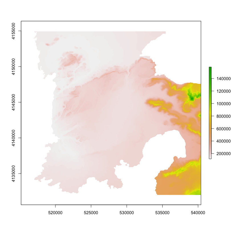
Location of the Milesian Peninsula: Miletos, Didyma and Panormos and changing topography
The Milesian peninsula is located on the west coast of modern Turkey, facing the Aegean sea. Today, the peninsula appears part of the mainland Turkish landmass, as a result of the extensive infilling of the former bay of Miletos by the alluvial delta created by sediment carried by the river Meander (modern Turkish Menderes or ancient Meandros).
sw_general_map <- function(dem, map_suffix="", roads="yes"){
  # Plot the background raster
  par(oma = c(0,0,0,0), xpd = TRUE)

  # Plot the basic terrain model
  col.palette = terrain.colors(30)
  image(dem,
        col = col.palette,
        xlab = "",
        ylab = ""
  )

  plot(outline_ancient_structures,
       border = "red",
       col = "transparent",
       lty = 1,
       lwd = 1.4,
       add = T
  )

  if (roads=="yes") plot(modern_major_roads,
       border = "black",
       col = "black",
       lty = 1,
       lwd = 1.1,
       alpha = 0.8,
       add = T
  )

  # Point text labels
  # pos=4 is to the right, 2=L, 1=below, 3=above
  text(coordinates(point_didyma_altar)[,1],
       coordinates(point_didyma_altar)[,2], "Didyma",
       pos= 4, offset=0.5, col="black", cex=1.3)
  text(coordinates(point_sacred_gate)[,1],
       coordinates(point_sacred_gate)[,2], "Miletos",
       pos= 4, offset=1.8, col="black", cex=1.3)
  text(coordinates(point_panormos)[,1],
       coordinates(point_panormos)[,2], "Panormos",
       pos= 2, offset=0.8, col="black", cex=1)

  if (roads=="yes")
  {
    legend("topright", # places a legend
         c("Modern roads"), # puts text in the legend
         lty=c(1), # appropriate symbols (lines)
         lwd=c(2.5),
         col=c("black"), # lines the correct color and width
         bg="white",
         box.col="black"
    )
  }

  # Title
  title(main=paste("Elevation model",map_suffix),
        outer = FALSE,
        cex.main = 1
  )
}

# Plot the map using cropped version of modern topography
sw_general_map(dem_modern, map_suffix=", using modern topography")
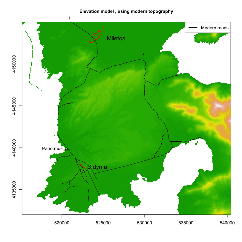
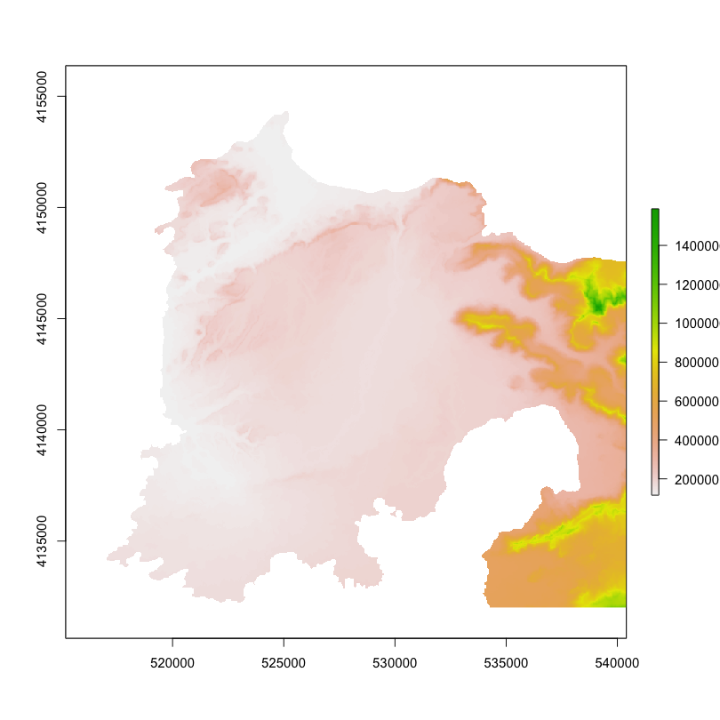
Up until sometime in the late Antique or early medieval period, however, the peninsula was only connected to the mainland via a relatively thin and mountainous strip in the south-east of the region. For this reason, the Milesian peninsula was, in ancient times, a true semi-island with most outside connections probably conducted by sea.
# Plot the map using cropped version of
# ancient topography
sw_general_map(dem_ancient, map_suffix = ", using ancient topography",
    roads = "no")
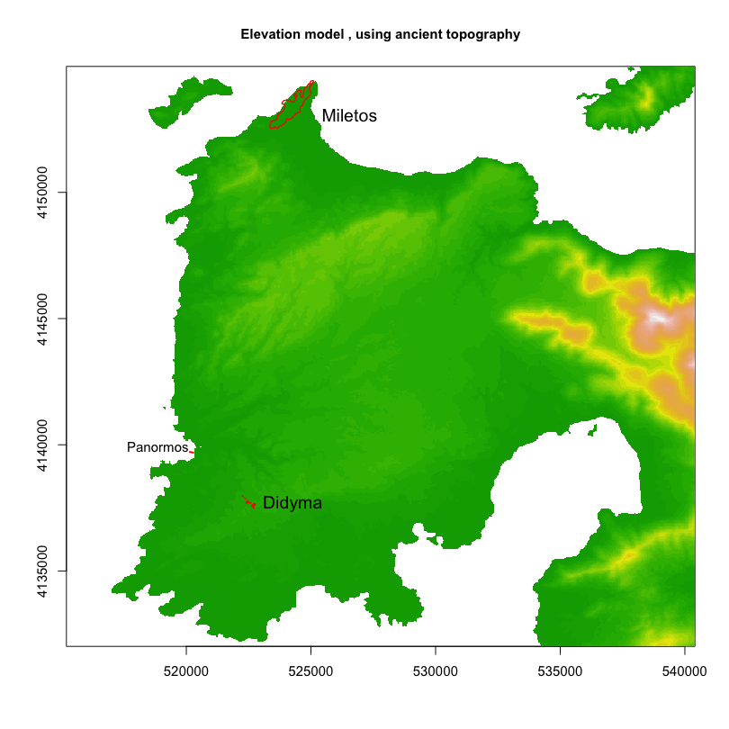
Within the half-island, settlements were presumably connected together with various internal tracks and roads, whether for driving animals, transporting goods or, as in the case of the Sacred Way, connecting important religious locales across Milesia.
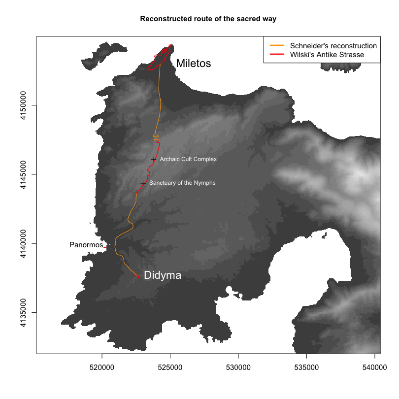
Reconstructions of the route of the Sacred Way
A proposed reconstruction of the entire route of the Sacred Way was published by Peter Schneider (1987) and has become the orthodox theory. Earlier, however, the coastal road was also assumed to be the most likely route, although Paul Wilski identified an ancient street running inland through the Akron hills.
The orthodox route of the sacred way
sw_general_place_labels <- function(place_lists = "DMPCN") {
    # A function to simplify the points labelled
    # by text in each map pos=4 is to the right,
    # 2=L, 1=below, 3=above
    if (grepl("D", place_lists)) {
        text(coordinates(point_didyma_altar)[,
            1], coordinates(point_didyma_altar)[,
            2], "Didyma", pos = 4, offset = 0.5,
            col = "white", cex = 1.5)
    }
    if (grepl("M", place_lists)) {
        text(coordinates(point_sacred_gate)[,
            1], coordinates(point_sacred_gate)[,
            2], "Miletos", pos = 4, offset = 1.8,
            col = "black", cex = 1.5)
    }
    if (grepl("P", place_lists)) {
        text(coordinates(point_panormos)[, 1],
            coordinates(point_panormos)[, 2],
            "Panormos", pos = 2, offset = 0.8,
            col = "black", cex = 1)
    }
    if (grepl("C", place_lists)) {
        text(coordinates(point_cult_complex)[,
            1], coordinates(point_cult_complex)[,
            2], "Archaic Cult Complex", pos = 4,
            offset = 0.7, col = "white", cex = 0.8)
    }
    if (grepl("N", place_lists)) {
        text(coordinates(point_nymph_complex)[,
            1], coordinates(point_nymph_complex)[,
            2], "Sanctuary of the Nymphs", pos = 4,
            offset = 0.7, col = "white", cex = 0.8)
    }
}

sw_general_reconstructions <- function(working_dem,
    primary_col = "orange", secondary_col = "red") {
    # Plot the background raster
    par(oma = c(0, 0, 0, 0), xpd = TRUE)

    # Plot the basic terrain model
    image(working_dem, col = gray.colors(20),
        xlab = "", ylab = "")

    plot(outline_ancient_structures, border = "red",
        col = "transparent", lty = 1, lwd = 1.3,
        add = T)

    plot(sacredway_schneider_south, col = primary_col,
        lty = 1, lwd = 1.1, add = T)
    plot(sacredway_schneider_north, col = primary_col,
        lty = 1, lwd = 1.1, add = T)
    plot(sacredway_wilski, col = secondary_col,
        lty = 1, lwd = 1.5, add = T)

    # Plot additional sites along the way
    plot(point_cult_complex, border = "black",
        add = T)
    plot(point_nymph_complex, border = "black",
        add = T)

    # Point text labels
    sw_general_place_labels()

    legend("topright", c("Schneider's reconstruction",
        "Wilski's Antike Strasse"), lty = c(1,
        1), lwd = c(2.5, 2.5), col = c("orange",
        "red"), bg = "white", box.col = "black")

    # Title
    title(main = paste("Reconstructed route of the sacred way"),
        outer = FALSE, cex.main = 1)
}

# Plot previous reconstructions with modern
# dem and default colours
sw_general_reconstructions(dem_ancient)
# A general settings for plotting maps for the rest of the analysis
sw_plot_map <- function(dem=NULL, overlay=NULL, col=NA,
      colNA=NA, alpha=1, legend=TRUE, title="",
      lohmann="", worldview="") {
  # Plot the background raster
  par(oma = c(0,0,0,0), xpd = TRUE)

  ## nb: it may be better to re-do this using spplot or
  ## ggplot in order to add more control and avoid axis/aspect
  ## issues with the spatial layers

  # Plot the basic terrain model
  if (!is.null(dem)) plot(dem,
       col = gray.colors(20),
       alpha = 0.6,
       legend = FALSE
       #yaxt="n",
       #xaxt="n"
  )

  # Plot satellite image if relevant
  if (worldview=="yes" && !is.null(worldview_multi)) {
    plotRGB(worldview_multi, r=5, g=3, b=2, stretch="lin", add=T)
  }

  # Plot the overlay (add if there is a dem, otherwise just plot direct)
  if (!is.null(overlay) && !is.null(dem)) plot(overlay,
       col = col,
       colNA = colNA,
       alpha = alpha,
       add = T
  )
  if (!is.null(overlay) && is.null(dem)) plot(overlay,
       col = col,
       colNA = colNA,
       alpha = alpha
  )

  plot(outline_ancient_structures,
       border = "red",
       col = "transparent",
       lty = 1,
       lwd = 1.3,
       add = T
  )

  # Plot the 'orthodox' routes as comparison
  plot(sacredway_schneider_south,
       col = "black",
       lty = 3,
       lwd = 0.9,
       add = T
  )
  plot(sacredway_schneider_north,
       col = "black",
       lty = 3,
       lwd = 0.9,
       add = T
  )
  plot(sacredway_wilski,
       col = "black",
       lty = 6,
       lwd = 1.1,
       add = T
  )

  if (lohmann=="yes") {
    points_subset <- crop(points_lohmann,dem)
    points_datedsubset <- subset(points_subset,
           (grepl("HEL", points_subset$Dating) |
            grepl("CLA", points_subset$Dating) |
            grepl("ROM", points_subset$Dating) |
            grepl("ARC", points_subset$Dating)) )
    plot(points_datedsubset,
       col = "red", # 36=a dark blue
       pch = 3,
       cex = 0.6,
       alpha = 0.7,
       add = T
    )
  }

  # Point text labels
  # pos=4 is to the right, 2=L, 1=below, 3=above
  text(coordinates(point_didyma_altar)[,1],
       coordinates(point_didyma_altar)[,2], "Didyma",
       pos= 4, offset=0.5, col="white", cex=1.5)
  text(coordinates(point_sacred_gate)[,1],
       coordinates(point_sacred_gate)[,2], "Miletos",
       pos= 4, offset=1.8, col="black", cex=1.5)
  text(coordinates(point_panormos)[,1],
       coordinates(point_panormos)[,2], "Panormos",
       pos= 2, offset=0.9, col="black", cex=1)

  # Axes
  #axis(2, hadj=0, col="red", cex=0.6) # left (north) axis
  #axis(1, hadj=0, col="red", cex=0.6) # bottom (east) axis

  # Legend text (just the orthodox route, plus ancient structures)
  legend("topright", # location
         c("Orthodox reconstruction","Ancient structures"), # legend
         lty=c(3,1), # symbols (lines)
         pch=c(NA,0), # symbols (over the line)
         lwd=c(1,1.3), # line width
         col=c("black","red"), # color and width
         bg="white",
         box.col="black"
  )
  txtkey <- c(paste("Sites recorded in Lohmann's ",
                        "extensive survey as Archaic, ",
                        "Classical, Hellenistic or ",
                        "Roman",sep=""))
  if (lohmann=="yes") {
    legend("bottomright",txtkey, pch=c(3),
           col=c("red"), cex=c(0.7),
           bg="white", box.col="black")
  }

  txtkey <- c("Base-map: Worldview-2 satellite image, ",
              "4 Sep 2011")
  if (worldview=="yes" && !is.null(worldview_multi)) {
    legend("topleft",txtkey,
           pch=c(3), col=c("white"),
           cex=c(0.6), bg="white", box.col="black")
  }

  # Title
  title(main=title,
        outer = FALSE,
        cex.main = 1,
        xlab = "east (UTM 36N)",
        ylab = "north"
  )
}
Explaining the analyses in geographical context
Create a conductance model (i.e. the inverse of a cost/friction/resistance surface)
Before any cost/friction-based analyses can be made, a model must be established to
enable subsequent calculations. The library used to make these calculations (gdistance)
relies on a conductance model (effectively the inverse of a cost/friction/resistance
model) in order to efficiently store the same network of relationships between cells. For
the purposes of the rest of this section, the phrase “resistance”‘” will be used as equivalent
to cost or friction in the sense of travel resistance across a geographical surface.
A varied and complex set of variables could theoretically be included in resistence-based models, depending on purpose of the analysis, but in this case, we are primarily interested in the effects of landscape change on the dominant factor in route creation (topography). In this work, then, topography (or rather slope) is used as the only variable to contribute to resistance.
The initial analysis for this study was conducted using ArcGIS’s PathDistance tool and the
procedures presented here were originally an attempt to replicate the same workflow. Note,
however, that differences in the way that PathDistance and gdistance are implemented means
that results are likely not to be identical. Whereas PathDistance uses a formula based on
a cost-raster (and then uses elevation values and any additional vertical or horizontal
factors) to multiply the resistence, gdistance relies on a transitionFunction to
create a conductance network. This transitionFunction must be manually designed by the
user. This means that anisotropic aspects (such as the additional distance travelled
vertically across a slope, and the variation in time/effort required to climb or descend
a slope) must be additionally programmed in.
A helpful example on how to use the gdistance package for modeling movement across a
terrain is provided under ‘Example 1: Hiking around Maunga Whau’ in the gdistance
package introductory vignette by Jacob van Etten (2014), R Package gdistance: Distances and Routes on Geographical Grids. Adaptation to this workflow were needed, however, for
the fact that the analysis described in the current paper includes an area of sea
(recorded as NoData or NA). More details on the workings of gdistance can be
found from the package documentation (link to CRAN).
Additionally, it is worth examining the discussion and review of least-cost procedures for archaeological applications in Irmela Herzog’s theoretical articles (e.g. Herzog 2013a, 2013b). She offers a range of alternative models which, while are not applied here, could offer alternative interpretative opportunities, including a model which is based on physiological experiments.
Transform elevation to slope: simple slope-as-resistence model
The simplest and often adequent initial model for resistence (or its inverse conductance) is based upon the slope of terrain.
Since slope by itself is not directly proportional to real-world costs (e.g. energy expenditure while walking, or time taken to walk up or down a given slope), various models have been proposed which are designed to provide more realistic or, often, more intuitive results to resistence-based analyses. The model presented here uses the ‘correction function’ used by Bell et al. (2002).
This simple model is flawed in certain details: first it is symmetrical, in that upslope and downslope are given equal weight (which is physiologically untrue), and second it is isotropic, in that it does not take account of the additional distance which must be covered by travelling vertically across the slope, as opposed to travelling horizontally across a flat terrain.
The second factor is likely to exaggerate the effects of slope through multiplication. The first may have a more ‘flattening’ effect for relatively gentle slopes for shortest paths (although it may have less effect on symmetrical analysis such as cost-corridors).
However, though testing is required, and the individual paths or corridors created might differ, it is unlikely the core results presented in this particular analysis would be radically different.
sw_simple_slope_conductance <- function(dem, dirs = 16,
    symm = FALSE) {
    # find slope
    slope <- terrain(dem, opt = "slope", unit = "radians",
        neighbors = 8)
    # slope <- tan(slope) * 100 # convert to
    # percent slope can be treated as a basic cost
    # but slope on its own is problematic, hence
    # the conversion formula, provided by Bell et
    slope <- tan(slope)/tan(pi/180)
    # gdistance requires a conductance (i.e.
    # 1/cost), but Inf conductance is problematic,
    # hence the +1
    slope <- (1/(1 + slope))
    # areas which are NA (e.g. the sea) should be
    # modelled as 0 conductance (Inf cost)
    slope[is.na(slope)] <- 0
    # the transition function sets the manner in
    # which cost is calculated between two
    # adjacent cells x[1] and x[2]
    tF <- function(x) {
        x[1] * x[2]
    }
    tr <- transition(slope, transitionFunction = tF,
        directions = dirs, symm = symm)
    # divide by the distance between cells
    tr <- geoCorrection(tr, type = "c")
    return(tr)
}
# Set alias to select which conductance
# function to use
sw_conductance <- function(dem, dirs = 16, symm = FALSE) {
    sw_simple_slope_conductance(dem, dirs = dirs,
        symm = symm)
}
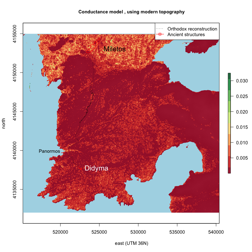
Such relative conductance models can be visualized as a raster map geographically:-
sw_plot_conductance <- function(dem, conductance,
map_suffix = "") {
# Create colour palette and plot
col.palette <- brewer.pal(10, "RdYlGn")
sw_plot_map(dem, overlay = raster(conductance),
col = col.palette, colNA = "lightblue",
alpha = 0.9, title = paste("Conductance model",
map_suffix))
}
# create sample symmetrical conductance using
# modern topography and plot as map
conductance_symm_mod <- sw_conductance(dem_modern,
dirs = 16, symm = TRUE)
sw_plot_conductance(dem_modern, conductance_symm_mod,
", using modern topography")
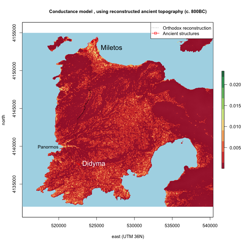
# create sample symmetrical conductance using
# ancient topography and plot as map
conductance_symm_anc <- sw_conductance(dem_ancient,
dirs = 16, symm = TRUE)
sw_plot_conductance(dem_ancient, conductance_symm_anc,
", using reconstructed ancient topography (c. 800BC)")
# other types of plot for testing purposes
# conductance_symm_mod
# image(transitionMatrix(conductance_symm_mod))
# conductance_symm_anc
This conductance matrix can now be used to perform various distance calculations
using gdistance functions.
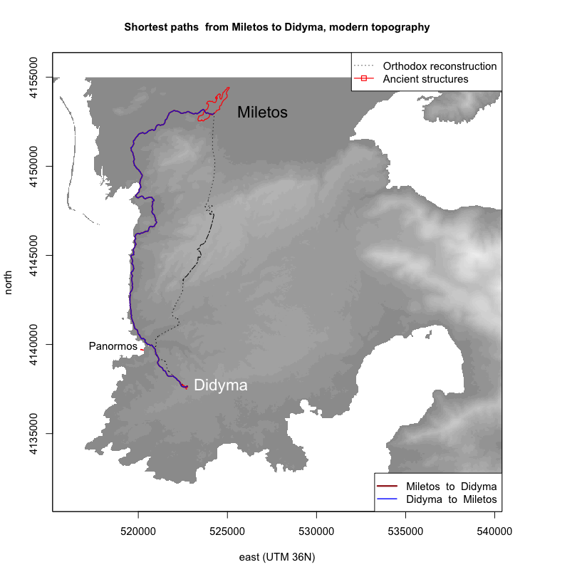
Create shortest paths between two points: Miletos and Didyma
Establishing the shortest path (often known as a least-cost-path) is perhaps the most commonly application of cost-surface techniques. It presents a single optimum calculation of the route with the lowest cumulated cost (or highest conductance), using a step-by-step algorithm to reach a particular destination point from a particular source point.
The shortestPath algorithm in the gdistance library uses Dijkstra’s algorithm (Dijkstra 1959). Additionally,
the path from A to B is usually not identical to the path from B to A, because of the assymetry of the model
and the algorithm used.
Here the shortest path from the so-called Sacred Gate complex at Miletos (the presumed start of the Sacred Way as it left the city walls) to the altar in front of the Temple of Apollo at Didyma is calculated as well as its inverse.
## using modern topography create assymetrical
## conductance transition
conductance_mod <- sw_conductance(dem_modern,
    dirs = 16, symm = FALSE)
# plot assymetric conductance (testing only)
# sw_plot_conductance(dem_modern,
# conductance_mod, ', using reconstructed
# modern topography')

# shortest path and its inverse
shortestpathMtoD_mod <- shortestPath(conductance_mod,
    point_sacred_gate, point_didyma_altar, output = "SpatialLines")
shortestpathDtoM_mod <- shortestPath(conductance_mod,
    point_didyma_altar, point_sacred_gate, output = "SpatialLines")

## using ancient topography create assymetrical
## conductance transition
conductance_anc <- sw_conductance(dem_ancient,
    dirs = 16, symm = FALSE)
# shortest path and its inverse
shortestpathMtoD_anc <- shortestPath(conductance_anc,
    point_sacred_gate, point_didyma_altar, output = "SpatialLines")
shortestpathDtoM_anc <- shortestPath(conductance_anc,
    point_didyma_altar, point_sacred_gate, output = "SpatialLines")
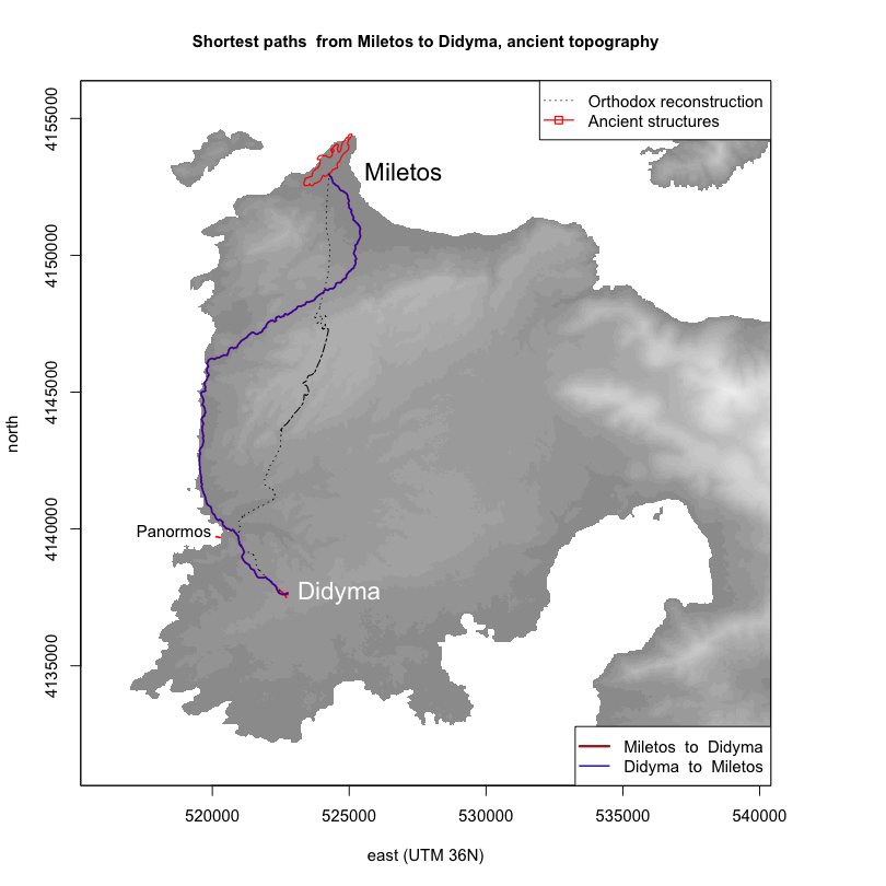
The geographical footprint of these shortest paths appears as follows:-
sw_plot_shortestpathpair <- function(dem, sp1,
    sp2, map_suffix = "", sp1_text = "A", sp2_text = "B") {
    sw_plot_map(dem, title = paste("Shortest paths",
        map_suffix))

    # Plot the two shorted (least-cost) paths
    plot(sp1, col = "brown", lty = "solid", lwd = 2,
        add = T)
    plot(sp2, col = "blue", lty = "solid", lwd = 1,
        add = T)

    # Legend text
    legend("bottomright", c(paste(sp1_text, " to ",
        sp2_text), paste(sp2_text, " to ", sp1_text)),
        lty = c(1, 1), pch = c(NA, NA), lwd = c(2.5,
            1.5), col = c("brown", "blue"), bg = "white",
        box.col = "black")

    # Label ends of lines? [WIP]!
    # text(coordinates(sp1)[,1],
    # coordinates(sp1)[,2], sp1_text)
    # text(coordinates(sp2)[,1],
    # coordinates(sp2)[,2], sp2_text)
}

sw_plot_shortestpathpair(dem_modern, shortestpathMtoD_mod,
    shortestpathDtoM_mod, " from Miletos to Didyma, modern topography",
    sp1_text = "Miletos", sp2_text = "Didyma")
sw_plot_shortestpathpair(dem_ancient, shortestpathMtoD_anc,
    shortestpathDtoM_anc, " from Miletos to Didyma, ancient topography",
    sp1_text = "Miletos", sp2_text = "Didyma")
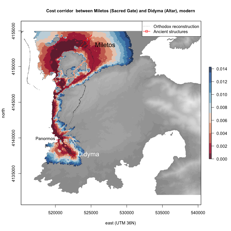
Create cost-corridor probability surface: Miletos to Didyma
Unitary least-cost-paths are problematic in as much as they represent arbitrary single routes and
do not give any sense of long-term variation. Alternative models providing a range of probabilities
have therefore been suggested, including cost corridors (normally the sum of two accumulated-cost-distance
surfaces, in gdistance this is called accCost) and, where there are more than two-nodes involved,
circuit-based modeling or resistance modeling (which in the case of gdistance is called
commuteDistance).
Creating a cost corridor between two points simply involves the sum or average of two accumulated cost surface calculations, one from each point.
sw_costcorridor <- function(conductance_symm,
    p1, p2) {
    accCostDistanceFromP1 <- accCost(conductance_symm,
        p1)
    accCostDistanceFromP2 <- accCost(conductance_symm,
        p2)

    # add the two cost distances together
    return(accCostDistanceFromP1 + accCostDistanceFromP2)
}

# modern
costCorridorBetweenMandD_mod <- sw_costcorridor(conductance_symm_mod,
    point_sacred_gate, point_didyma_altar)
# costCorridorBetweenMandD_mod
plot(costCorridorBetweenMandD_mod)

# ancient meander
costCorridorBetweenMandD_anc <- sw_costcorridor(conductance_symm_anc,
    point_sacred_gate, point_didyma_altar)
# costCorridorBetweenMandD_anc
plot(costCorridorBetweenMandD_anc)
The resultant raster needs to be reclassified in order to visualize corridors and exclude areas not of interest, for example, as follows:-
sw_costcorridor_scale <- function(conductance_symm,
    p1, p2, rescale = TRUE, max = 1, percentile = 1) {
    accCostDistanceFromP1 <- accCost(conductance_symm,
        p1)
    accCostDistanceFromP2 <- accCost(conductance_symm,
        p2)

    # add the two cost distances together
    costCorridor = accCostDistanceFromP1 + accCostDistanceFromP2

    # first need to exclude Inf accumulate cost by
    # setting to NA
    costCorridor[is.infinite(costCorridor)] = NA

    # function to rescale cell values between 0
    # and 1 from Tim Assal
    # http://www.timassal.com/?p=859
    rasterRescale <- function(r) {
        ((r - cellStats(r, "min"))/(cellStats(r,
            "max") - cellStats(r, "min")))
    }

    # rescale to between 0 and 1 if rescale set to
    # TRUE
    costCorridor_reclass <- costCorridor
    if (rescale)
        costCorridor_reclass <- rasterRescale(costCorridor)

    # Exclude certain percentage of results e.g.
    # 0.1 = is 10% percentile
    if (percentile < 1)
        max <- quantile(costCorridor_reclass,
            probs = c(percentile), na.rm = TRUE)

    # Exclude all values above a certain value
    # e.g. 0.08
    if (max < 1)
        costCorridor_reclass[costCorridor_reclass >
            max] = NA

    return(costCorridor_reclass)
}

## 20% percentile selects a relatively
## reasonable modern
costCorridorBetweenMandD_mod <- sw_costcorridor_scale(conductance_symm_mod,
    point_sacred_gate, point_didyma_altar, percentile = 0.25)
# ancient
costCorridorBetweenMandD_anc <- sw_costcorridor_scale(conductance_symm_anc,
    point_sacred_gate, point_didyma_altar, percentile = 0.25)

## output information about reclassified
## costCorridor costCorridorBetweenMandD_mod
The resultant raster can be visualised geographically as follows:-
sw_plot_costcorridor <- function(dem, costcorridor,
map_suffix = "", lohmann = "", worldview = "") {
# Create palette and plot map
col.palette <- brewer.pal(10, "RdBu")
# col.palette = heat.colors(30)
ifelse((worldview == "yes"), alpha <- 0.5,
alpha <- 0.8)
sw_plot_map(dem, costcorridor, col = col.palette,
alpha = alpha, title = paste("Cost corridor",
map_suffix), lohmann = lohmann, worldview = worldview)
if (worldview == "yes") {
outline <- rasterToPolygons(costcorridor >
0.6, dissolve = TRUE)
plot(outline, col = NA, border = "white",
lty = 1, lwd = 0.9, add = T)
}
}
sw_plot_costcorridor(dem_modern, costCorridorBetweenMandD_mod,
" between Miletos (Sacred Gate) and Didyma (Altar), modern")
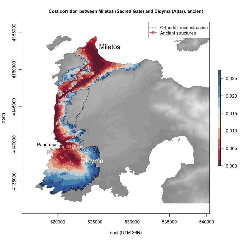
sw_plot_costcorridor(dem_ancient, costCorridorBetweenMandD_anc,
" between Miletos (Sacred Gate) and Didyma (Altar), ancient")
Focus region: the harbour region of Panormos
# plot maps side-by-side (nrows, ncols)
# uncomment this line if two charts should be
# plotted side-by-side par(mfrow=c(1,2))
Focusing the analysis around the uncertain segment near Panormos
Using the basic models outlined above, we will focus the analysis on the region around the harbor of Panormos. Here, certain features of the landscape suggest the possibility that the coastline may have lain further inland than the current map suggests, which has consequences for the possible resistence/cost corridors and pathways which may have been favored.
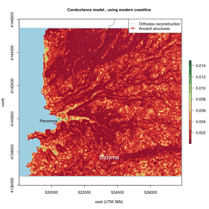
Create a conductance model
# create sample symmetrical conductance using
# modern topography and plot as map
conductance_symm_mod <- sw_conductance(dem_wilski_modern,
dirs = 16, symm = TRUE)
sw_plot_conductance(dem_wilski_modern, conductance_symm_mod,
", using modern coastline")
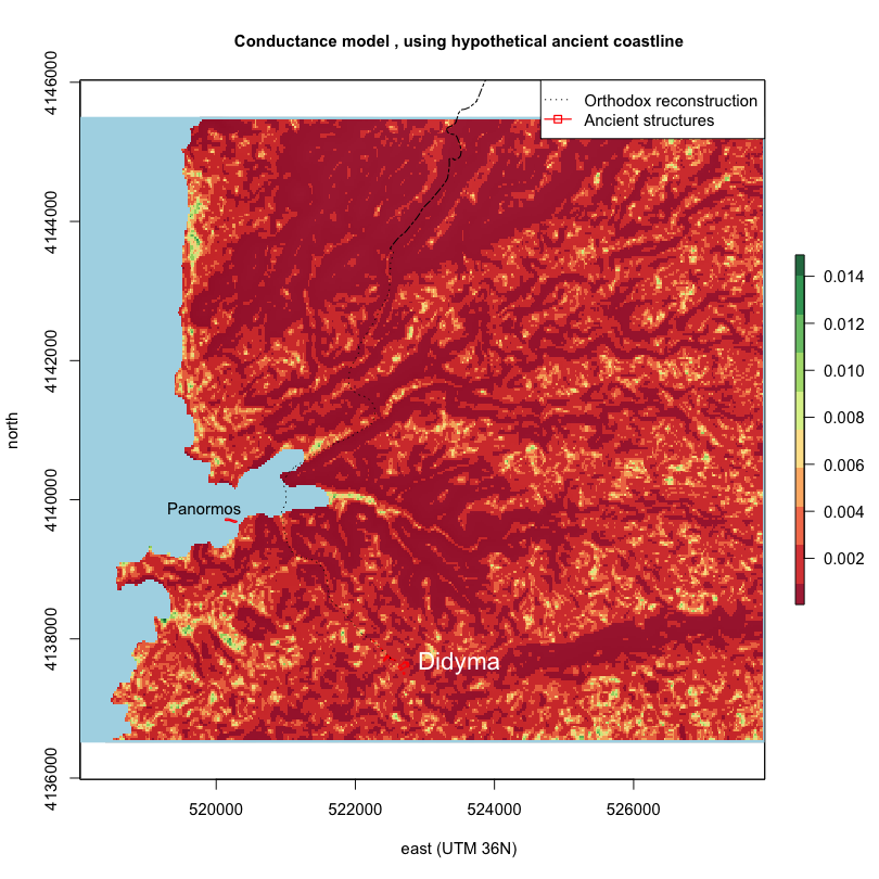
# create sample symmetrical conductance using
# ancient topography and plot as map
conductance_symm_anc <- sw_conductance(dem_wilski_prealluv,
dirs = 16, symm = TRUE)
sw_plot_conductance(dem_wilski_prealluv, conductance_symm_anc,
", using hypothetical ancient coastline")
Create shortest path lines
We will assume here that Wilksi’s Antike Strasse remains part of the sacred way for most of it’s history and
therefore start our cost calculations from the point at which it leaves the Akron hills and becomes difficult
to trace archaeologically (point_road_leaving_akron).
## using modern topography create assymetrical
## conductance transition
conductance_mod <- sw_conductance(dem_wilski_modern,
    dirs = 16, symm = FALSE)
# shortest path and its inverse
shortestpathAtoD_mod <- shortestPath(conductance_mod,
    point_road_leaving_akron, point_didyma_altar,
    output = "SpatialLines")
shortestpathDtoA_mod <- shortestPath(conductance_mod,
    point_didyma_altar, point_road_leaving_akron,
    output = "SpatialLines")

## using ancient topography create assymetrical
## conductance transition
conductance_anc <- sw_conductance(dem_wilski_prealluv,
    dirs = 16, symm = FALSE)
# shortest path and its inverse
shortestpathAtoD_anc <- shortestPath(conductance_anc,
    point_road_leaving_akron, point_didyma_altar,
    output = "SpatialLines")
shortestpathDtoA_anc <- shortestPath(conductance_anc,
    point_didyma_altar, point_road_leaving_akron,
    output = "SpatialLines")

# write line to file
sw_write_sl_as_gml <- function(sl, filepath, nn) {
    df <- data.frame(len = sapply(1:length(sl),
        function(i) gLength(sl[i, ])))
    rownames(df) <- sapply(1:length(sl), function(i) sl@lines[[i]]@ID)
    writeOGR(SpatialLinesDataFrame(sl, data = df),
        filepath, nn, driver = "GML", overwrite_layer = T)
}
sw_write_sl_as_gml(shortestpathAtoD_anc, paste("_Outputs",
    "shortestpathAtoD_anc.gml", sep = "/"), "shortestpathAtoD_anc")

# Plot the maps
sw_plot_shortestpathpair(dem_wilski_modern, shortestpathAtoD_mod,
    shortestpathDtoA_mod, " from Antike Strasse to Didyma, modern coastline",
    "Akron", "Didyma")
sw_plot_shortestpathpair(dem_wilski_prealluv,
    shortestpathAtoD_anc, shortestpathDtoA_anc,
    " from Antike Strasse to Didyma, hypothetical ancient coastline",
    "Akron", "Didyma")
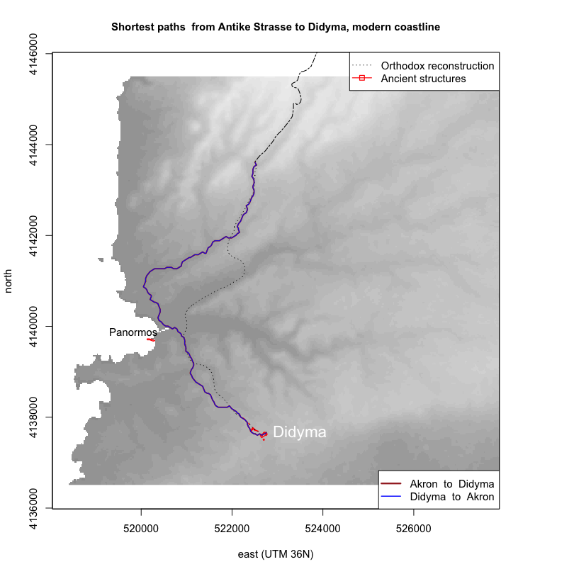
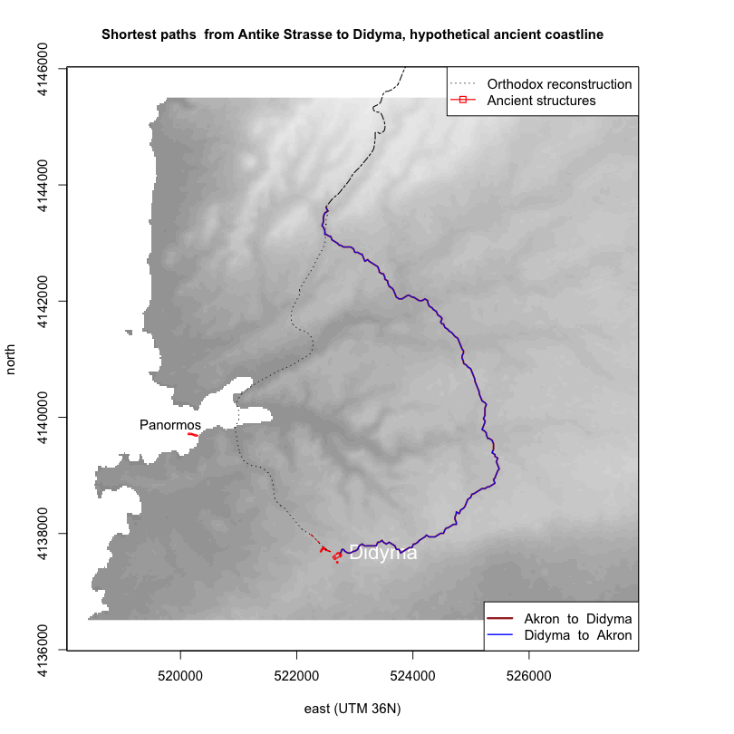
It is clear here, using the simple_slope_conductance model, that the effect of a relatively small
change in the shape of the harbour can have a big effect on the shortest path: before alluviation,
the shortest path lies far in-land, re-filling the harbour to roughly the modern (1960s) line, makes
the shortest path follow a route quite close to the orthodox reconstruction.
Create cost-corridors
Again the shortest path line is in some senses more arbitrary since such a model cannot hope to predict an actual path accurately. The cost-corridor, however, offers a more nuanced probability layer.
# modern
costCorridorBetweenAandD_mod <- sw_costcorridor_scale(conductance_symm_mod,
    point_road_leaving_akron, point_didyma_altar,
    percentile = 0.2)
# ancient
costCorridorBetweenAandD_anc <- sw_costcorridor_scale(conductance_symm_anc,
    point_road_leaving_akron, point_didyma_altar,
    percentile = 0.2)

# output information about reclassified
# costCorridor
costCorridorBetweenAandD_mod
## class       : RasterLayer
## dimensions  : 292, 400, 116800  (nrow, ncol, ncell)
## resolution  : 24.6, 30.8  (x, y)
## extent      : 518044, 527884, 4136509, 4145503  (xmin, xmax, ymin, ymax)
## coord. ref. : +proj=utm +zone=35 +datum=WGS84 +units=m +no_defs +ellps=WGS84 +towgs84=0,0,0
## data source : in memory
## names       : layer
## values      : 0, 0.05932335  (min, max)
# plot as maps
sw_plot_costcorridor(dem_wilski_modern, costCorridorBetweenAandD_mod,
" between Antike Strasse and Didyma, modern coastline",
lohmann = "yes")
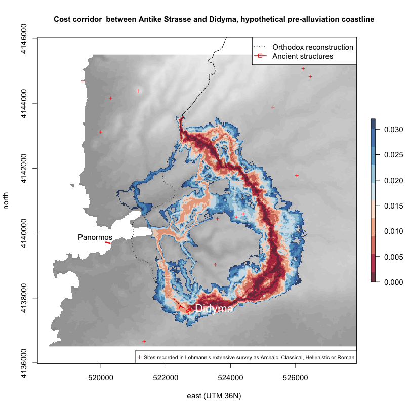
sw_plot_costcorridor(dem_wilski_prealluv, costCorridorBetweenAandD_anc,
" between Antike Strasse and Didyma, hypothetical pre-alluviation coastline",
lohmann = "yes")
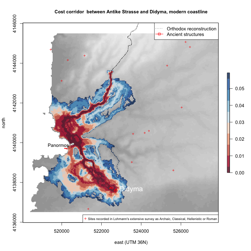
The post-alluviation (modern) cost-corridor from Akron to Didim runs to the coast, with the highest probability zone containing the orthodox reconstruction. An alternative corridor to the orthodox route is offered in the first section (when the cost-corridor skips a turn and heads straight to the coast) and around half-way (where it would be possible to travel round to the west of a set of low hills behind modern Mavişehir instead of along the modern main road).
The pre-alluviation cost-distance shows that the highest probability of movement runs far in land of the post-alluviation situation, albeit with 2 much lower probability corridors running somewhere halfway between the post-alluvial corridor and pre-alluvial maximum. In either case, the result is very similar to less nuanced shortest-path analysis: a difference in the topography around the harbor can make a substantial change to the probability of a route based incidentally or intentionally on slope cost travelling through the Panormos harbour area or much further in land.
The pre-alluviation corridor (i.e. hypothetically ancient or original route) also approaches the sanctuary at Didyma area to the front of the Apollo temple.
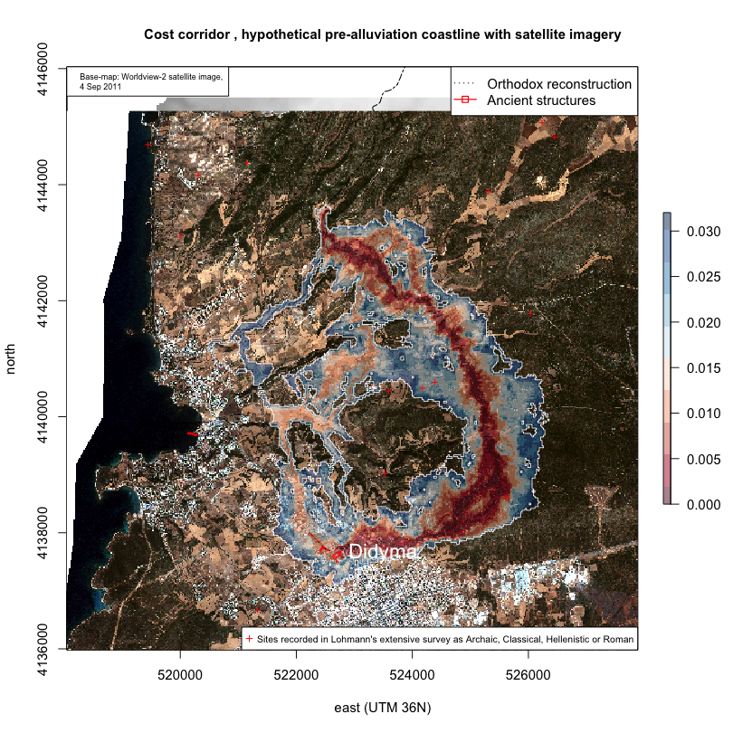
As the location of sites from Lohmann’s extensive survey show, this in-land area, although relatively unused in the modern day (shown by the modern satellite imagery), actually has a number of sites dating to between ca. 800BC and AD400.
# modern plot as maps
sw_plot_costcorridor(dem_wilski_prealluv, costCorridorBetweenAandD_anc,
    ", hypothetical pre-alluviation coastline with satellite imagery",
    lohmann = "yes", worldview = "yes")
Concluding comments
The variation in the shortest path and cost corridors created by potential changes in the shoreline support the possibility that, if travel cost was a factor in at least parts of the routing of the Sacred Way, routes other than the orthodox reconstruction could have been favoured at different periods, as the affordances of the landscape changed through time.
Although these are merely heuristic models, the lend weight to the suggestion, based on epigraphical evidence, that a change of route could have been made following the in-filling of the harbour, perhaps during the late Hellenistic or Roman era. Geomorphological data may be able to provide better empirical evidence for the exact dating of any such alluviation process.
Acknowledgements
This analysis was presented in an earlier form at a conference organized by the British Institute at Ankara and Ankara University in 2011, Pathways of Communication. The authors are grateful for the chance to discuss our results and ideas in that forum. Encouragement to convert the original GIS analysis into a more robust reproducible RMarkdown form was provided by Néhémie Strupler. Technical help and suggestions to help make the analysis function correctly using gdistance was provided by Jacob van Etten and Chris English. The responsibility for remaining errors of fact and interpretation belongs to the authors.
Bibliography
Bell, T., Wilson, A., and Wickham, A. 2002. “Tracking the Samnites: landscape and communications routes in the Sangro Valley, Italy.” American Journal of Archaeology 106 (2): 169-186.
Dijkstra, E. 1959. “A Note on Two Problems in Connexion with Graphs.” Numerische Mathematik 1(1): 269–271.
Grewe, K., 2004. “Alle Wege führen nach Rom – Römerstraßen im Rheinland und anderswo.” In „Alle Wege führen nach Rom“, Internationales Römerstraßenkolloquium Bonn, edited by H. Koschik, Materialien zur Bodendenkmalpflege im Rheinland, 16. 9-42.
Herzog, I. 2013a. The Potential and Limits of Optimal Path Analysis. In Computational Approaches to Archaeological Spaces, edited by A. Bevan and M Lake. London: Left Coast Press. 179-212.
Herzog, I. 2013b. Theory and practice of cost functions. In Fusion of Cultures. Proceedings of the 38th Annual Conference on Computer Applications and Quantitative Methods in Archaeology, Granada, Spain, April 2010, edited by F. Contreras, M. Farjas and F.J. Melero. British Archaeological Reports International Series 2494, Oxford: Archaeopress. 375-82.
Herzog, I. 2013c. “Review of Least Cost Analysis of Social Landscapes. Archaeological Case Studies [Book],” Internet Archaeology 34: http://dx.doi.org/10.11141/ia.34.7
Llobera, M., Sluckin, T.J., 2007. “Zigzagging: Theoretical insights on climbing strategies.“” Journal of Theoretical Biology 249: 206-217.
Marotte, R. (nd). http://robbymarrotte.weebly.com/blog/category/resistance-distance
Minetti, A. E., Moia, C., Roi, G. S., Susta, D., Ferretti, G., 2002. “Energy cost of walking and running at extreme uphill and downhill slopes.” Journal of Applied Physiology 93: 1039-1046.
Müllenhoff, M. 2005. Geoarchäologische, sedimentologische und morphodynamische Untersuchungen im Mündungsgebiet des Büyük Menderes (Mäander), Westtürkei. Marburg: Marbuger Geographische Gesellschaft.
Schneider, P. 1987. “Zur Topographie der Heiligen Straße von Milet nach Didyma,”” Archäologischer Anzeiger: 101–129
van Etten, J. 2014. R Package gdistance: Distances and Routes on Geographical Grids, https://cran.r-project.org/web/packages/gdistance/vignettes/gdistance1.pdf
van Etten J. and Hijmans, R. 2010. “A Geospatial Modelling Approach Integrating Archaeobotany and Genetics to Trace the Origin and Dispersal of Domesticated Plants.“” PLoS ONE, 5(8), e12060.

Route modeling of the Sacred Way between Miletos and Didyma
by Toby C. Wilkinson, Anja Slawisch
is licensed under a
Creative Commons Attribution 4.0 International License.